| Everything Oracle | Home | Everything Oracle |
| Essbase | Cube | Creation | |||||
| Creating an Essbase Cube from a Relational Data Source | |||||||
| Tutorial Overview |
Before starting this tutorial, read the article on “Understanding Multidimensional Databases”, which explains the data set we’ll use and shows the nine basic cube views that can be constructed from it. Also read the article on “Integration Services Architecture”, which provides some conceptual background for the steps involved in Essbase cube creation.
The assumptions that we’ll make in this tutorial are that the Shared Services, the Integration Services, the Essbase Server, and the Administration Services processes are up and running.
We’ll first create a Data Source by creating a new schema in an Oracle database. We’ll run a script to create a set of tables and to load some sample data. We’ll also create a schema to hold the OLAP Metadata Catalog.
Then we’ll create two ODBC data sources, one to connect to the database containing the Data Source and one to connect to the database containing the OLAP Metadata Catalog (as we’ll use the same database for both purposes, all we really need is a single ODBC data source, but we’ll create two to make it clear which ODBC data source is been used for which purpose during cube creation).
Next we’ll create the OLAP Metadata Catalog – a set of empty tables in the relational database.
Next we’ll login to Integration Services, providing one login to allow Integration Services to connect to the OLAP Metadata Catalog, and another to allow it to connect to the Essbase Server.
Next we’ll create the OLAP Model and save it to the OLAP Metadata Catalog.
Next we’ll create, on the basis of the OLAP Model, an OLAP Metaoutline and save it to the OLAP Metadata Catalog.
Next we’ll load the data from the Data Source into an Essbase Cube using the information stored in the OLAP Metadata Catalog.
Finally, we’ll examine the cube data using the Administration Services Console to make sure that the data has been loaded correctly.
Now, having “talked the talk”, let’s “walk the walk”!
| Create the Data Source and OLAP Metadata Catalog Schemas |
In this section, we’ll create the schema for the Data Source and load it with sample data. We’ll also create the schema that will be used to contain the OLAP Metadata Catalog.
Login to SQL*Plus as user “system” and create a new schema for the OLAP Metadata Catalog:
create user metacat identified by <password>;
grant connect, resource to metacat;
and for the Data Source:
create user sales identified by <password>;
grant connect, resource to sales;
Create a SQL script, called “sales.sql”, by cutting and pasting the following text (note, this is the same data set that we discussed in the “Understanding Multidimensional Databases” article):
-- DROP TABLES ON RE-RUN
DROP TABLE sales;
DROP TABLE customers;
DROP TABLE products;
-- CREATE CUSTOMERS TABLE
CREATE TABLE customers (
customer_id number(6)
constraint pk_cst primary key,
customer_name varchar2(40),
customer_region varchar2(10)
);
-- CREATE PRODUCTS TABLE
CREATE TABLE products (
product_id number(6)
constraint pk_prd primary key,
product_name varchar2(40),
product_category varchar2(30)
);
-- CREATE SALES TABLE
CREATE TABLE sales (
customer_id number(6)
constraint fk_sal_cst references
customers ( customer_id ),
product_id number(6)
constraint fk_sal_prd references
products ( product_id ),
sales_quantity number(4),
sales_value number(8,2)
);
-- CREATE CUSTOMERS
INSERT INTO customers VALUES ( 1, 'Brudenbacker', 'US' );
INSERT INTO customers VALUES ( 2, 'Smithers', 'US' );
INSERT INTO customers VALUES ( 3, 'Contraine', 'EMEA' );
-- CREATE PRODUCTS
INSERT INTO products VALUES ( 1, 'Disk Drive', 'Electronics' );
INSERT INTO products VALUES ( 2, 'Drill', 'Hardware' );
INSERT INTO products VALUES ( 3, 'Circular Saw', 'Hardware' );
-- CREATE SALES
INSERT INTO sales VALUES ( 1, 1, 10, 2500 );
INSERT INTO sales VALUES ( 1, 2, 5, 1000 );
INSERT INTO sales VALUES ( 1, 3, 10, 1000 );
INSERT INTO sales VALUES ( 1, 3, 20, 2000 );
INSERT INTO sales VALUES ( 2, 2, 20, 4000 );
INSERT INTO sales VALUES ( 2, 3, 30, 3000 );
INSERT INTO sales VALUES ( 3, 1, 10, 2500 );
INSERT INTO sales VALUES ( 3, 2, 20, 4000 );
INSERT INTO sales VALUES ( 3, 3, 10, 1000 );
Note, that the sales data has one missing customer-product combination and one duplicated customer-product combination.
Login to SQL*Plus as user “sales” and run script “sales.sql”. Commit the data and exit SQL*Plus.
We now have two schemas: one is empty, “metacat”, and the other is populated with tables and data, “sales”.
| Create the ODBC Data Sources |
In this section we’ll create two ODBC data sources, one to connect to the database containing the Data Source and one to connect to the database containing the OLAP Metadata Catalog (we only need one ODBC data source, but by creating two it will help us to distinguish how they are used for different purposes by Integration Services).
Navigate to “Start => Control Panel => Administrative Tools => Data Sources (ODBC)”. Double-click on the “Data Sources (ODBC)” item. When the “ODBC Data Source Administrator” window appears, select the “System DSN” tab:
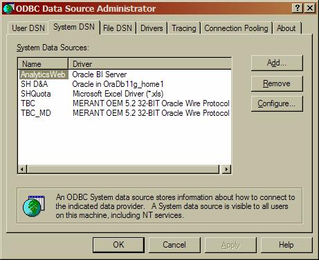
ODBC Data Source Administrator Window
Press the “Add” button. In the “Create New Data Source” window, select the “MERANT OEM 5.2 32-BIT Oracle Wire Protocol” driver, and then press “Finish”:
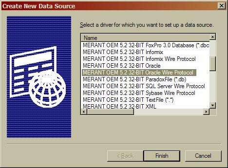
Create New Data Source Window
In the “ODBC Oracle Wire Protocol Driver Setup” window enter the following information: Data Source Name: “Sales”; Description: “Connects to Data Source”; Host: “<name of machine hosting Oracle database>”; Port Number: “1521”; SID: “orcl” (or your Oracle database SID if it’s different). Then press the “Test Connect” button:
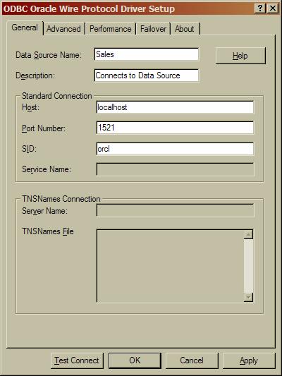
ODBC Oracle Wire Protocol Driver Setup Window
In the “Logon to Oracle Wire Protocol” window enter the schema name for the Data Source, “sales”, the corresponding password, and then press the “OK” button:
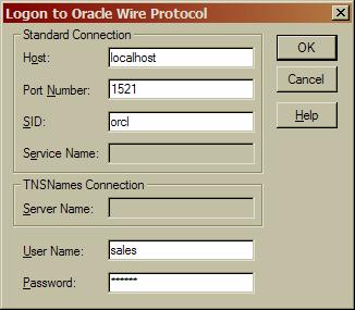
Logon to Oracle Wire Protocol Window
The “Test Connect” window appears showing that a connection has been established:
Test Connect Window
Press the “OK” button to return to the “ODBC Oracle Wire Protocol Driver Setup” window, and then press “OK” to return to the “System DSN” tab.
Repeat the process for the OLAP Metadata Catalog schema, “metacat”, using the appropriate values: Data Source Name: “OLAP Metadata Catalog”; and Description: “Connect to OLAP Metadata Catalog”. The “ODBC Data Source Administrator” window should now show the two new ODBC connections:
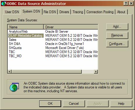
ODBC Data Source Administrator Window
Press “OK” to exit.
We now have two ODBC data sources, “Sales” and “OLAP Metadata Catalog”, allowing us to connect to the databases containing the “sales” and “metacat” schemas respectively.
| Create the OLAP Metadata Catalog |
In this section, we’ll create the OLAP Metadata Catalog as a set of tables in schema “metacat”.
Navigate to “Start => All Programs => Hyperion => Integration Services => Integration Services Console”. Press the “Close” and “Cancel” buttons in any pop-up windows that appear, so that the “Essbase Integration Services Console” main window is displayed:
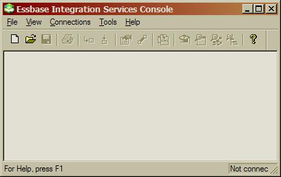
Essbase Integration Services Console Window
Navigate to “Tools => Create Catalog”. Enter the following values: Server Name: “<name of machine hosting integration services>”; Catalog ODBC DSN: “OLAP Metadata Catalog”; Code Page: “English (Latin1)”; User Name: “metacat”; Password: “<password>”. Deselect the “Show this dialog at Startup” radio button. Press the “Create” button. A pop-up window appears, indicating that catalog creation has been successful:
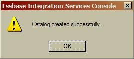
Catalog Creation Successful Window
Press the “OK” button, followed by “Close”. Leave the “Essbase Integration Services Console” window open.
If you login to SQL*Plus as user “metacat” and select “object_type” and “object_name” from “user_objects” you’ll see the indexes and tables that comprise the newly created OLAP Metadata Catalog:
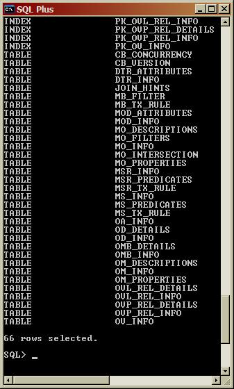
OLAP Metadata Catalog Database Objects
We now have an empty OLAP Metadata Catalog, which can be used to hold OLAP Models and OLAP Metaoutlines.
| Create the OLAP Model |
In this section, we’ll create an OLAP Model as a star schema representing the relational metadata stored in our Data Source schema, “sales”.
Logging In
From the “Essbase Integration Services Console” window navigate to “File => New”. The Login window appears. This window contains three sections corresponding to three of the links in the diagram in the “Integration Services Architecture” article. The “Essbase Integration Services” section provides logon details for the OLAP Metadata Catalog; the “Essbase” section provides logon details for the Essbase Server, and the “Shared Services” section provides logon details for Shared Services (in the pop-up invoked by clicking on the button).
You’ll need to provide logon details for the OLAP Metadata Catalog in order to create the OLAP Model and the OLAP Metaoutline, and you’ll need to provide logon details for the Essbase Server in order to create and populate the Essbase cube.
Enter values in the “Essbase Integration Services” section as follows: Server: “<name of machine hosting integration services>” (“localhost” is not acceptable), OLAP Metadata Catalog: “OLAP Metadata Catalog”; Code Page: “English (Latin1)”; User Name: “metacat”; Password: “<password>”.
Enter values in the “Essbase” section as follows: Server: “<name of machine hosting essbase server>” (“localhost” is not acceptable); User Name: “<essbase user name>”; Password: “<essbase user password>” (ask your Hyperion administrator for these values, if necessary).
When completed, the “Login” window should be similar to the following:
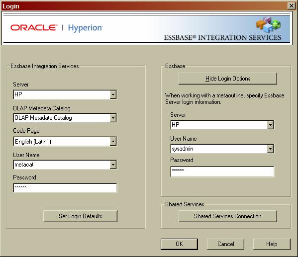
Login Window
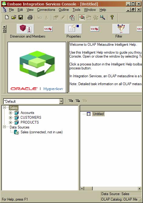
Press “OK” to continue, and the “Welcome” window will appear:
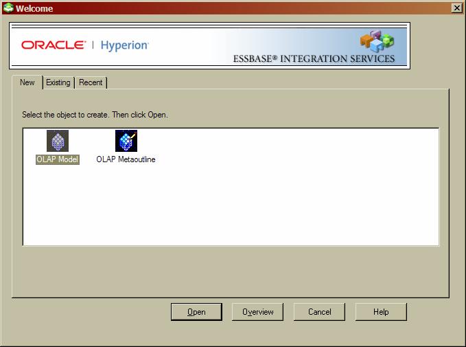
Welcome Window
This window allows you to create and edit OLAP Models and OLAP Metaoutlines in the context OLAP Metadata Catalog.
Select the “OLAP Model” icon and press the “Open” button. To create a new OLAP Model you need to connect to a data source, so the “Data Source” window will appear. Specify the logon details for the “sales” schema as follows: Data Source: “Sales”; Code Page: “English (Latin1)”; User Name: “sales”; Password: “<password>”:
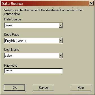
Data Source Window
Press the “OK” button and the OLAP Model Editor window will appear (if this is your first access to the Data Source expect a very long wait before the window appears):
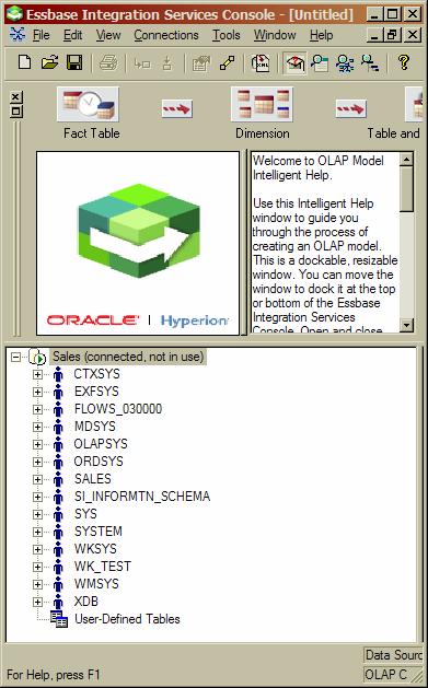
OLAP Model Editor Window
If the large cube icon and the “Welcome to OLAP Model Intelligent Help” pane are not displayed, navigate to “Tools” and click on “Intelligent Help”.
Click on the “Fact Table” icon.
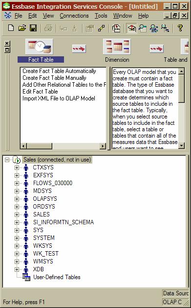
OLAP Model Editor Window
Intelligent Help is ... well ... quite helpful. The icons listed horizontally, “Fact Table”, “Dimension”, “Table and Column Properties”, “Hierarchy”, and “Finish” represent steps in the OLAP Model creation process (not all are necessary). For each of these steps a list of tasks that may be required is presented in the top left hand pane, together with a set of instructions on how to carry out the context task in the top right hand pane.
Selecting a Fact Table
Select the “Create Fact Table Manually” task. Expand the “SALES” and then “TABLES” nodes in the bottom left hand pane, and drag table “SALES.SALES” to the bottom right hand pane (note, if you have forgotten to create the tables in the “sales” schema – so that the schema is empty – then the “sales” schema will not be listed). When asked if you wish to create a “Time dimension” press “No”, and when asked if you wish to create an “Accounts dimension” press “Yes”:
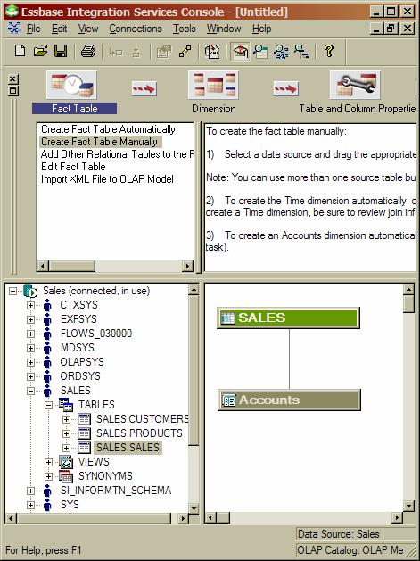
Fact Table and Accounts Dimension
Remember that the “sales” table in schema “sales” is the source for our fact table since it contains the two measures, “sales_quantity” and “sales_value”. We don’t need a time dimension since our fact table doesn’t contain a “Time ID” column.
The “Accounts” dimension that we’ve created is not a true dimension. It’s needed when the fact table contains multiple measures. Its main purpose is in specifying additive measures. Since Hyperion is primarily aimed at the financial sector, fact table measures will often represent amounts in a specified unit of currency. If the measures are “additively compatible” in this manner, then it’s often of interest to ask questions about sums of measures as well as about individual measures. The Accounts dimension facilitates questions of this type.
Creating Dimensions
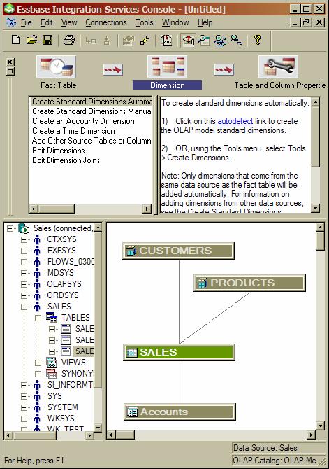
Our next task is to create standard dimensions corresponding to our “Products” and “Customers” tables. Click on the “Dimensions” icon and on the “Create Standard Dimensions Automatically” task:
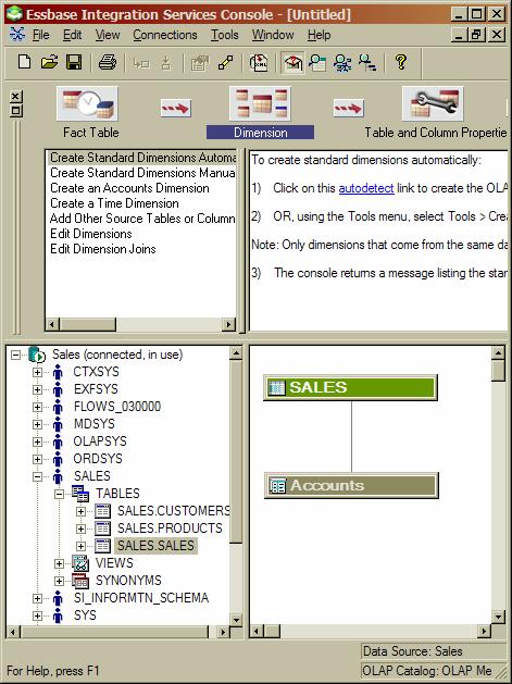
Dimension Focus
Click on the “autodetect” link in the top right hand pane. Integration Services will examine the foreign-key links defined between the fact table and any master dimension tables to determine the dimensions:
Autodetection of Standard Dimensions
Note, if a dimension table had, in turn, a master table (corresponding to a snowflake schema), then Integration Services would include the indirect master table in the dimension, but would give it the same name as the direct master.
Note, if you haven’t created foreign-key constraints between the fact table and its direct master tables, then Integration Services won’t “discover” the dimensions – it does not match foreign-key column names against primary-key column names to identify table joins.
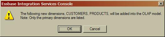
Press the “OK” button:
Customers and Products Dimensions Added
Creating Hierarchies
Select the “Hierarchy” icon and then the “Create Standard Hierarchy Manually” task from the top left hand pane:
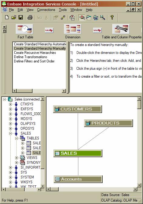
Creating Standard Hierarchies Manually
Select the “Customers” dimension table in the diagram in the bottom right hand pane. Right-click and select “Properties” from the pop-up window that appears. Select the “Hierarchies” tab, and then press the “Add” button. The “Edit Hierarchy” window appears:
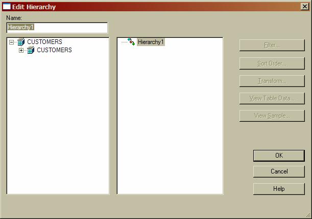
Edit Hierarchy Window
Expand the “CUSTOMERS” node in the left hand pane. Double-click first the “CUSTOMER_REGION” item and then the “CUSTOMER_NAME” item:
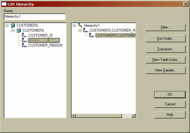
Customers Hierarchy Added
Note, since there can be multiple customers in a region, “Customer Region” appears above “Customer Name” in the hierarchy.
Press “OK” twice. Now repeat the process with the “Products” dimension table, this time placing “PRODUCT_CATEGORY” above “PRODUCT_NAME” in the hierarchy.
Verify and Save
Select “File => Verify” from the menu:
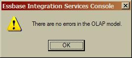
OLAP Model Verified
and press “OK”. Then select “File => Save” from the menu. Enter a value of “Sales” in the “OLAP Model Name” field:
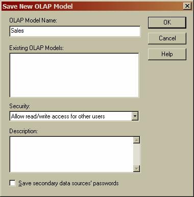
Saving the OLAP Model
Press “OK”, followed by “File => Close” to exit the OLAP Model Editor.
Our OLAP Model is now complete. We have identified the fact table, the dimension tables, and for each dimension table we’ve identified the columns that are of interest and arranged them in a hierarchy.
| Create the OLAP Metaoutline |
In this section, we’ll create an OLAP Metaoutline based on the OLAP Model that we created in the previous section.
Opening the Editor
From the “Essbase Integration Services Console” window navigate to “File => New”. The “Welcome” window will appear as before (you’re still logged in so the “Login” window does not appear this time). Select the “OLAP Metaoutline” icon, and then select the “Sales” OLAP Model from the drop-down list:
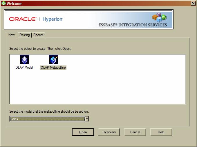
Welcome Window
Press the “Open” button. The “Data Source” window appears. Enter the same values as before: Data Source: “Sales”; Code Page: “English (Latin1)”; User Name: “sales”; Password: “<password>” and press “OK”. The OLAP Metaoutline Editor appears:
OLAP Metaoutline Editor
This editor works in the same way as the OLAP Model editor.
Selecting Cube Dimensions
Select the “Dimensions and Members” icon and then the “Create Standard Dimensions Automatically” task:
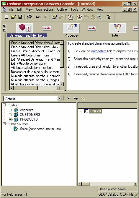
Creating Standard Dimensions Automatically
Click on the “autodetect” link in the top right hand pane. In the “Existing Hierarchies” window press the “Select All” button:
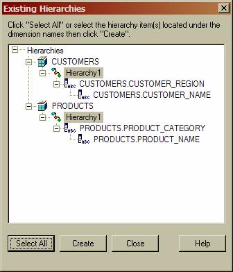
Selecting Hierarchies
Here, we’re selecting from the hierarchies in the OLAP Model those that we want to incorporate into the Essbase cube.
Press the “Create” button to return to the OLAP Metaoutline editor.
One thing that is not done automatically in the previous task is to add the “non-standard” measure dimension, “Accounts”. To add this dimension, select “Create Standard Dimensions Manually”. First drag the “Accounts” node in the bottom left hand pane to the bottom right hand pane, and place it below the two hierarchies that are already present. Then expand the “Accounts” node in the bottom left hand pane so that the column names are visible. Drag, in turn, the “SALES_QUANTITY” and “SALES_VALUE” measure columns to the newly created “Accounts” node in the bottom right hand pane:
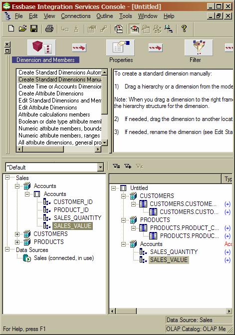
Accounts Dimension Added
Verify and Save
Select “File => Verify” from the menu. The pop-up window will indicate that the OLAP Metaoutline is valid for aggregate storage. Press “OK”. Select “File => Save” from the menu. Enter a value of “Sales” for the “Metaoutline Name” field, and press “OK”. Leave the OLAP Metaoutline editor open.
Our OLAP Metaoutline is now complete. We have identified the hierarchies to be used when the Essbase cube is created.
Set the Storage Model
Select the “Sales” node in the bottom right hand pane. Right-click and select “Properties” from the pop-up window that appears. Click on the “Data Storage Model” tab:
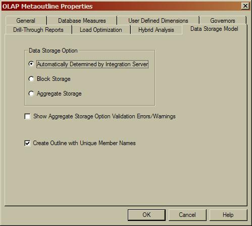
Data Storage Model
Make sure the “Automatically Determined by Integration Server” radio button is selected within the “Data Storage Option” section (from the “Verify” process we already know that the OLAP Metaoutline is valid for aggregate storage). Press the “OK” button and then “File => Save”. Leave the OLAP Metaoutline editor open.
| Load Members and Data |
In this section, we’ll create the Essbase cube and load data into it.
From within the OLAP Metaoutline editor select the “Finish” icon, and then the “Member or Data Load” task. Select “Outline => Member and Data Load” from the menu. In the “Essbase Application and Database” window, enter the following values: Application Name: “Sales” and Database Name: “Sales”. Make sure “None” is selected as the value for the “Calc Scripts” radio button:
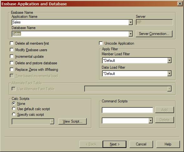
Essbase Application and Database Window
Press “Next” and then “Finish”. The “Member and Data Load” in progress window appears. When the load is complete a pop-up window appears:
Cube Loaded Successfully
Press “OK”. Examine the entries in the “Member and Data Load” window:
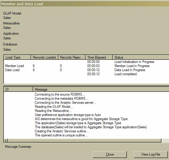
Member and Data Load Window
In the top pane note that six member records and eight data load records were loaded. The “Products” and “Customers” tables each contain three distinct rows which accounts for the six members. The sales table contains nine rows, but two of these correspond to the same product and customer values, so that there are eight distinct combinations of product and customer in the sales table (measure column values for non-distinct combinations are summed or aggregated when preparing the Essbase cube).
In the bottom pane note that the aggregate storage model has been selected. Also in the bottom pane:
Member and Data Load Window
you can see the three select statements that were sent to the “sales” schema in order to populate the Essbase cube. The selects from “Customers” and “Products” select all rows. The select from “sales” involves a sum over the measure column values as expected. Note that the two measures have been added to the Accounts dimension.
Note, that whereas the top pane indicated that six member records were loaded, the bottom pane indicates that 10 members were loaded, five from each table. Now each table contains three distinct values for the column corresponding to the lowest level in the hierarchy (“Customer Name” and “Product Name”), and two distinct values for the column corresponding to the next highest level in the hierarchy (“Customer Region” and “Product Category”), which makes five distinct members for each dimension.
Press “Close” and then “File => Exit”.
| Viewing the Cube Data |
In this section, we’ll examine the data in the Essbase cube to make sure it’s all present and accounted for.
Navigate to “Start => All Programs => Hyperion => Administration Services => Start Administration Services Console” and enter the following values in the “Essbase Administration Services Login” window: Administration Services: “<name of machine hosting essbase server>”; Username: “<essbase user name>”; Password: “<essbase user password>”:
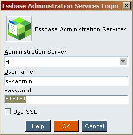
Administration Services Login Window
Press “OK”. Navigate to “Enterprise View => Essbase Servers => <essbase server> => Applications => Sales => Sales => Outline”. Right-click, and in the pop-up window that appears select “View”:
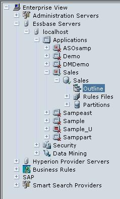
Sales Application and Database
Expand the nodes that appear in the right hand pane:
Sales Outline
We can see the five members corresponding to each of the two standard dimensions arranged in hierarchical order, plus the two measures in the Accounts dimension.
Select the “Sales” database in the left hand pane, right-click, and select “Preview data” from the pop-up window that appears:
Accounts Measures Added Together
A value of “21135.0” is shown at the intersection of the “Products” column and the “Customers” row. The sum of “sales_quantity” column values equals “135” and the sum of “sales_value” column values equals “21000”. The “Accounts” dimension treats these two measures as though they were compatible and adds them together, which in the present case makes no sense. Select the “Account” header, and click on the “Zoom In” icon (the magnifying glass with the plus sign). This operation drills down on the “Accounts” dimension, splitting the two measures apart:
All Customers versus All Products
Zoom in on the “Customers” header and we now have sales values and quantities for all products displayed by “Customer Region”.
Customer Regions versus All Products
Zoom in on the “Products” header and we now have sales values and quantities displayed by “Customer Region” and “Product Category” in the form of a pivot table:
Customer Regions versus Product Categories
Zoom in on “US”, “EMEA”, “Electronics”, and “Hardware”:
Essbase Cube
Now we have drilled down as far as we can go. The base members are displayed for both customers and products, and we can see the complete set of data held in the Essbase cube for each measure.
Note, the data value of “#MISSING” at the intersection of the “Smithers” and “Disk Drive” members. This arises because we have no row in our “sales” table for this combination of customer name and product name.
If you check the nine views in the master table in the “Understanding Multidimensional Databases” article, you’ll see that the five views shown above are a subset of the nine. The other views can be obtained by drilling down first on the “Products” dimension. Use the “Zoom Out” icon to drill up, and then drill down again.
| Everything Oracle | Home | Everything Oracle |
Copyright © 2007-2015 PWG Consulting, All Rights Reserved